


Superconductivity of Solid Hydrogen under Extreme Pressure
-
摘要: 氢元素在常压下具有最简单的晶体结构和物理性质。随着压强增加,氢单质发生相变,由绝缘体转变为金属,被称为金属氢。数值模拟表明,金属氢具有高温超导电性,因此,金属氢研究也被称为高压物理领域的“圣杯”课题。利用基于密度泛函理论的第一性原理计算方法,对固体氢在极端高压(0.5~5.0 TPa)下的结构和超导电性开展了系统研究。研究结果表明:固体氢的高压相变序列为I41/amd→oC12→cI16;对于同一种结构,随着压强增加,电声耦合系数减小,费米面处电子态密度减小,特征振动频率增加,超导转变温度发生小幅变化;在2.0 TPa压强下,固体氢的超导转变温度高达418 K(库伦赝势经验值μ*=0.10)。研究工作将为金属氢及其超导电性的后续理论和实验研究提供参考。Abstract: Hydrogen has the simplest crystal structure and physical properties at ambient pressure. As the pressure increases, hydrogen undergoes phase transition from insulator to metal, which being called metallic hydrogen. The numerical calculations also indicate that metallic hydrogen has high-temperature super-conductivity, thus the metal hydrogen is also known as the holy grail of physics subject. In this paper, the structural phase transition and superconducting transition temperature (Tc) of solid hydrogen under extreme high pressure 0.5–5.0 TPa were studied by first principles based on density functional theory, which may provide knowledge reserved for subsequent theoretical and experimental studies of metallic hydrogen and its superconductivity. The results show that the phase transition sequence of solid hydrogen under extreme high pressure is: I41/amd→oC12→cI16. For the same structure, with the increase of pressure, the electron-phonon-induced interaction decreases, the density of electronic states at the Fermi surface decreases, the vibration frequency increases, and the superconducting transition temperature changes. When the pressure is 2.0 TPa, the oC12 structure of solid hydrogen can obtain the highest Tc of 418 K (coulomb pseudopotential parameter μ*=0.10). This work provides a reference for further theoretical and experimental research on metallic hydrogen and its superconductivity.
-

图 1 (a) 极端高压下各结构相对于I41/amd相固体氢的焓差随压强的变化,(b) 考虑零点振动能后极端高压下各结构相对于oC12相固体氢的焓差随压强的变化
Figure 1. (a) Calculated enthalpies of various structures as a function of pressure with respect to I41/amd structure; (b) calculated enthalpies of various structures with the inclusion of ZPE as a function of pressure with respect to the oC12 structure
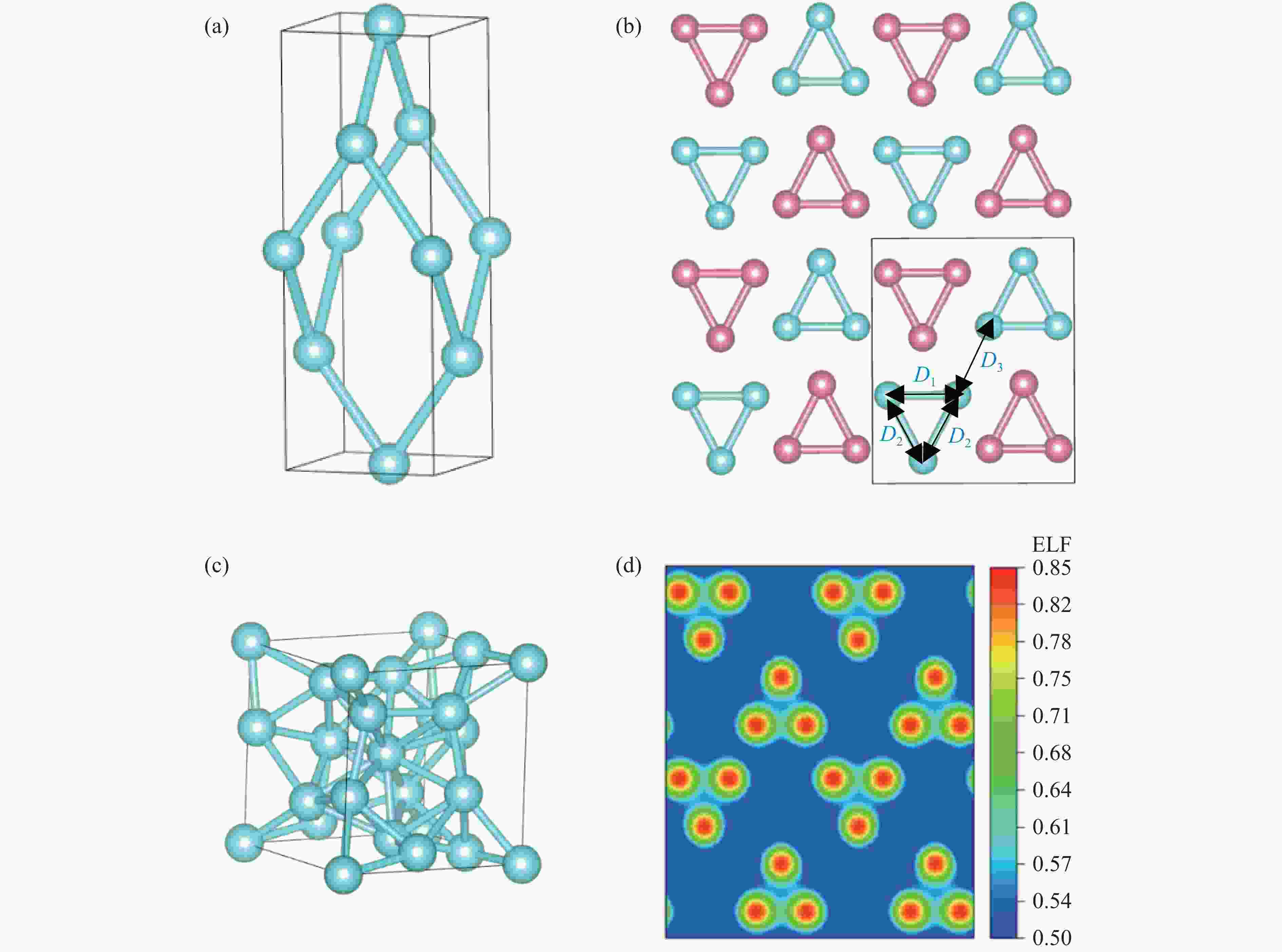
图 2 3.0 TPa下I41/amd相(a)、oC12相(b)(不同颜色的原子代表不同层)、cI16相(c)固体氢的结构和oC12相电子局域函数(d)(均使用VESTA绘制[28])
Figure 2. I41/amd structure (a), oC12 structure (b) (spheres of different colors indicate different layers), and cI16 structure (c), and ELF profile of the oC12 structure (d) at 3.0 TPa (All structures and the ELF profile were drawn by using VESTA[28])
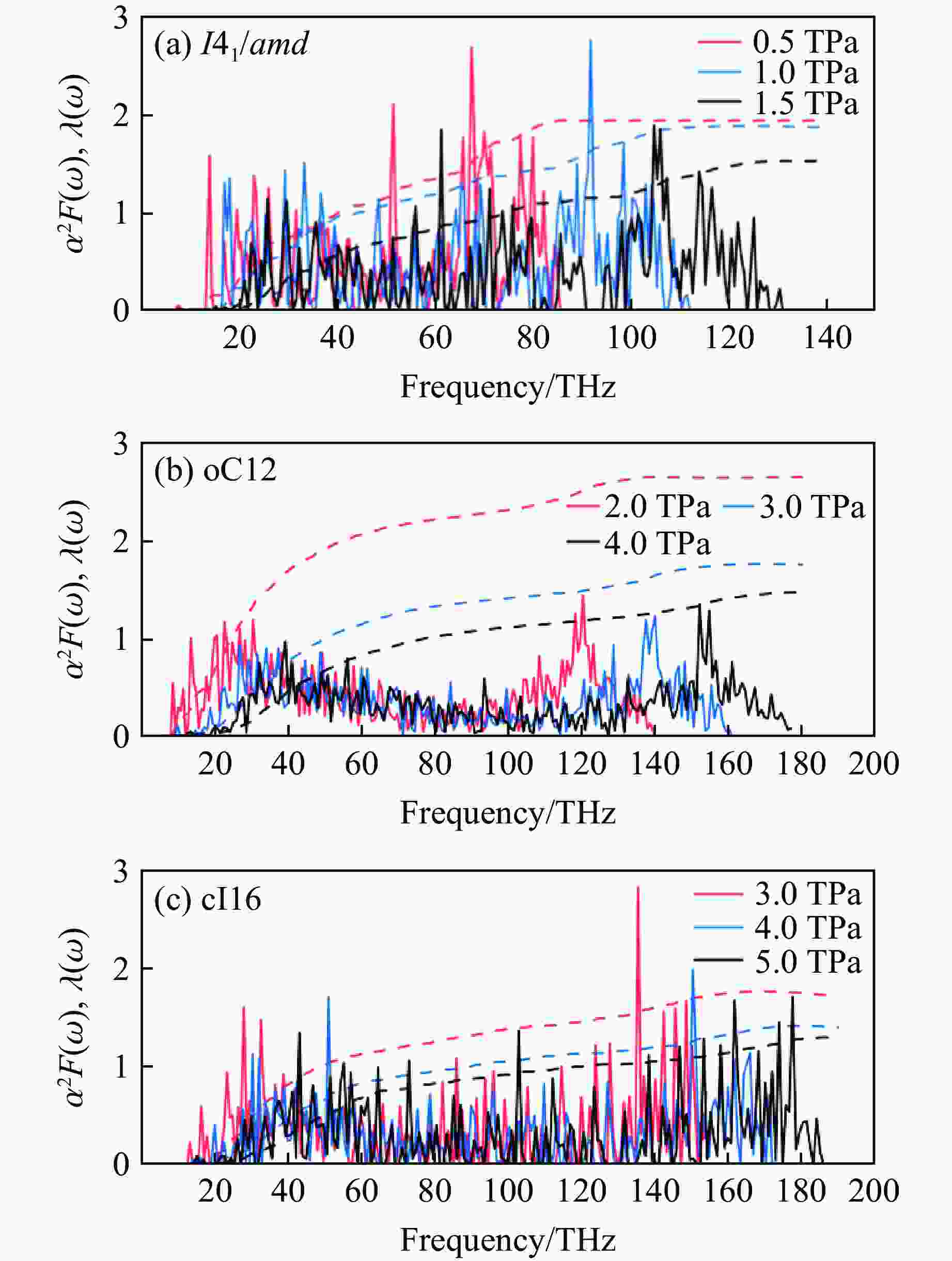
图 3 不同压强下各结构谱函数α2F(ω)及电声耦合系数λ(ω)
Figure 3. Éliashberg spectral function α2F(ω) together with the electron-phonon integral λ(ω) at different pressures
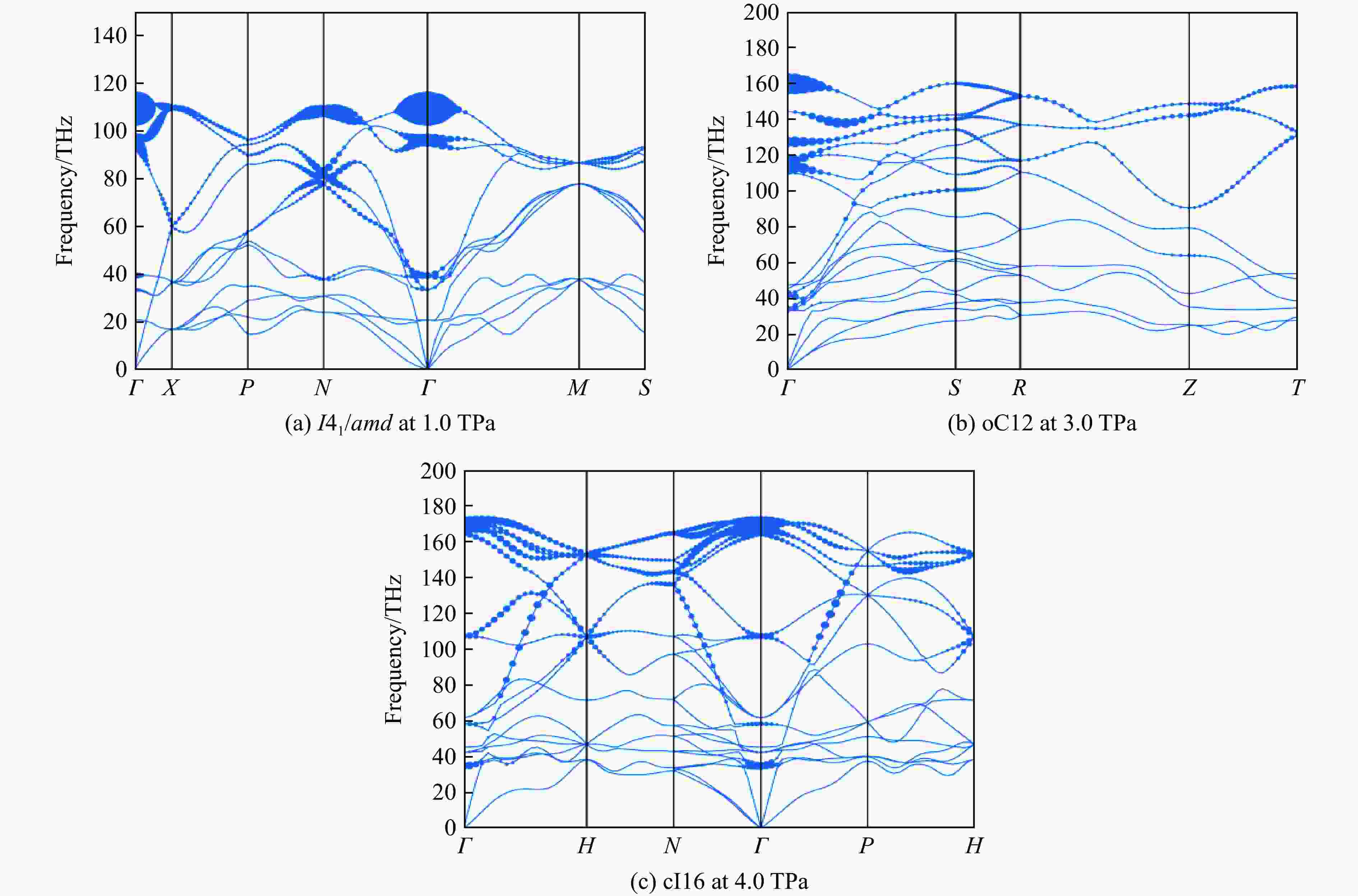
图 4 不同压强下各结构的声子谱
Figure 4. Phonon dispersion curves of each structure at different pressures
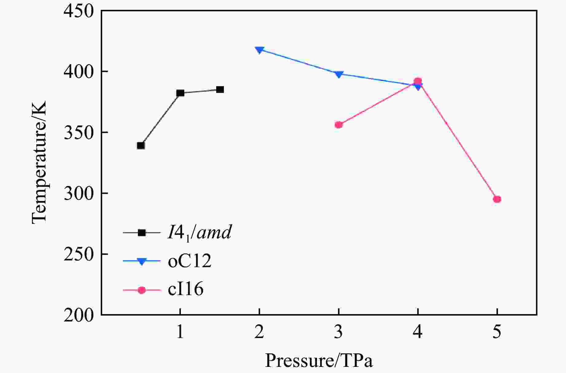
图 5 各结构的超导转变温度随压强的变化(μ*=0.10)
Figure 5. Superconducting critical temperatures Tc of each structure with μ*=0.10
表 1 优化后的结构参数
Table 1. Optimized structural parameters
Structure p/TPa Lattice parameters Atomic coordinates (fractional) I41/amd 1.0 a=b=1.067 9 Å, c=2.993 9 Å,
α=β=γ=90°H1(4a) 0 1 0 oC12(Cmcm) 3.0 a=0.947 9 Å, b=2.812 3 Å, c=2.319 0 Å,
α=β=γ=90°H1(8f) 0.500 0 0.140 5 0.580 7 H2(4c) 0.500 0 0.595 6 1.250 0 cI16($I\overline4 3d $) 4.0 a=b=c=1.929 3 Å, α=β=γ=90° H1(16c) 0.955 5 0.455 5 0.044 5  下载: 导出CSV
表 2 不同压强下各结构的超导转变温度及超导计算中的重要参数
Table 2. Calculated superconducting parameters and the superconducting transition temperature for I41/amd, oC12, cI16 under different pressures
Structure p/TPa λ ωlog/K $N_{E_{\rm{F}}} $/
(states·Ry−1/atom)Tc/K μ*=0.10 μ*=0.13 μ*=0.17 I41/amd 0.5 1.94 1 784.5 0.23 339 307 280 1.0 1.87 2 039.0 0.20 382 354 320 1.5 1.53 2 539.5 0.19 385 348 310 oC12 2.0 2.65 1 580.2 0.18 418 391 356 3.0 1.77 2 324.7 0.16 398 356 318 4.0 1.48 2 822.3 0.14 388 353 312 cI16 3.0 1.73 2 303.0 0.16 356 345 307 4.0 1.42 2 782.6 0.14 392 362 322 5.0 1.27 3 159.0 0.13 295 258 217
下载: 导出CSV
-
[1] WIGNER E, HUNTINGTON H B. On the possibility of a metallic modification of hydrogen [J]. The Journal of Chemical Physics, 1935, 3(12): 764–770. doi: 10.1063/1.1749590 [2] PICKARD C J, NEEDS R J. Structure of phase Ⅲ of solid hydrogen [J]. Nature Physics, 2007, 3(7): 473–476. doi: 10.1038/nphys625 [3] MCMAHON J M, CEPERLEY D M. Ground-state structures of atomic metallic hydrogen [J]. Physical Review Letters, 2011, 106(16): 165302. doi: 10.1103/PhysRevLett.106.165302 [4] EREMETS M I, DROZDOV A P, KONG P P, et al. Semimetallic molecular hydrogen at pressure above 350 GPa [J]. Nature Physics, 2019, 15(12): 1246–1249. doi: 10.1038/s41567-019-0646-x [5] DIAS R P, SILVERA I F. Observation of the Wigner-Huntington transition to metallic hydrogen [J]. Science, 2017, 355(6326): 715–718. doi: 10.1126/science.aal1579 [6] LOUBEYRE P, OCCELLI F, DUMAS P. Synchrotron infrared spectroscopic evidence of the probable transition to metal hydrogen [J]. Nature, 2020, 577(7792): 631–635. doi: 10.1038/s41586-019-1927-3 [7] ASHCROFT N W. Metallic hydrogen: a high-temperature superconductor? [J]. Physical Review Letters, 1968, 21(26): 1748–1749. doi: 10.1103/PhysRevLett.21.1748 [8] CUDAZZO P, PROFETA G, SANNA A, et al. Ab initio description of high-temperature superconductivity in dense molecular hydrogen [J]. Physical Review Letters, 2008, 100(25): 257001. doi: 10.1103/PhysRevLett.100.257001 [9] YAN Y, GONG J, LIU Y H. Ab initio studies of superconductivity in monatomic metallic hydrogen under high pressure [J]. Physics Letters A, 2011, 375(9): 1264–1268. doi: 10.1016/j.physleta.2011.01.045 [10] MAKSIMOV E G, SAVRASOV D Y. Lattice stability and superconductivity of the metallic hydrogen at high pressure [J]. Solid State Communications, 2001, 119(10/11): 569–572. [11] SZCZȨS̀NIAK R, JAROSIK M W. The superconducting state in metallic hydrogen under pressure at 2 000 GPa [J]. Solid State Communications, 2009, 149(45/46): 2053–2057. [12] MCMAHON J M, CEPERLEY D M. High-temperature superconductivity in atomic metallic hydrogen [J]. Physical Review B, 2011, 84(14): 144515. doi: 10.1103/PhysRevB.84.144515 [13] LIU H Y, WANG H, MA Y M. Quasi-molecular and atomic phases of dense solid hydrogen [J]. The Journal of Physical Chemistry C, 2012, 116(16): 9221–9226. doi: 10.1021/jp301596v [14] KRESSE G, FURTHMÜLLER J. Efficient iterative schemes for ab initio total-energy calculations using a plane-wave basis set [J]. Physical Review B, 1996, 54(16): 11169–11186. doi: 10.1103/PhysRevB.54.11169 [15] BLÖCHL P E. Projector augmented-wave method [J]. Physical Review B, 1994, 50(24): 17953–17979. doi: 10.1103/PhysRevB.50.17953 [16] PERDEW J P, BURKE K, ERNZERHOF M. Generalized gradient approximation made simple [J]. Physical Review Letters, 1996, 77(18): 3865–3868. doi: 10.1103/PhysRevLett.77.3865 [17] MONKHORST H J, PACK J D. Special points for Brillouin-zone integrations [J]. Physical Review B, 1976, 13(12): 5188–5192. doi: 10.1103/PhysRevB.13.5188 [18] TOGO A, CHAPUT L, TADANO T, et al. Implementation strategies in phonopy and phono3py [J]. Journal of Physics: Condensed Matter, 2023, 35(35): 353001. doi: 10.1088/1361-648X/acd831 [19] TOGO A. First-principles phonon calculations with phonopy and phono3py [J]. Journal of the Physical Society of Japan, 2023, 92(1): 012001. doi: 10.7566/JPSJ.92.012001 [20] GIANNOZZI P, BARONI S, BONINI N, et al. QUANTUM ESPRESSO: a modular and open-source software project for quantum simulations of materials [J]. Journal of Physics: Condensed Matter, 2009, 21(39): 395502. doi: 10.1088/0953-8984/21/39/395502 [21] MIGDAL A B. Interaction between electrons and lattice vibrations in a normal metal [J]. Soviet Physics JETP, 1958, 34(7): 996–1001. [22] ÉLIASHBERG G M. Interactions between electrons and lattice vibrations in a superconductor [J]. Soviet Physics JETP, 1960, 11(3): 696–702. [23] SCALAPINO D J, SCHRIEFFER J R, WILKINS J W. Strong-coupling superconductivity.Ⅰ [J]. Physical Review, 1966, 148(1): 263–279. doi: 10.1103/PhysRev.148.263 [24] VIDBERG H J, SERENE J W. Solving the Eliashberg equations by means of N-point Padé approximants [J]. Journal of Low Temperature Physics, 1977, 29(3/4): 179–192. [25] HANFLAND M, SYASSEN K, CHRISTENSEN N E, et al. New high-pressure phases of lithium [J]. Nature, 2000, 408(6809): 174–178. doi: 10.1038/35041515 [26] GREGORYANZ E, LUNDEGAARD L F, MCMAHON M I, et al. Structural diversity of sodium [J]. Science, 2008, 320(5879): 1054–1057. doi: 10.1126/science.1155715 [27] MCMAHON M I, GREGORYANZ E, LUNDEGAARD L F, et al. Structure of sodium above 100 GPa by single-crystal X-ray diffraction [J]. Proceedings of the National Academy of Sciences of the United States of America, 2007, 104(44): 17297–17299. [28] MOMMA K, IZUMI F. VESTA 3 for three-dimensional visualization of crystal, volumetric and morphology data [J]. Journal of Applied Crystallography, 2011, 44(6): 1272–1276. doi: 10.1107/S0021889811038970 [29] ALLEN P B, DYNES R C. Transition temperature of strong-coupled superconductors reanalyzed [J]. Physical Review B, 1975, 12(3): 905–922. doi: 10.1103/PhysRevB.12.905 [30] DROZDOV A P, EREMETS M I, TROYAN I A, et al. Conventional superconductivity at 203 kelvin at high pressures in the sulfur hydride system [J]. Nature, 2015, 525(7567): 73–76. doi: 10.1038/nature14964 [31] MA L, WANG K, XIE Y, et al. High-temperature superconducting phase in clathrate calcium hydride CaH6 up to 215 K at a pressure of 172 GPa [J]. Physical Review Letters, 2022, 128(16): 167001. doi: 10.1103/PhysRevLett.128.167001 [32] KONG P P, MINKOV V S, KUZOVNIKOV M A, et al. Superconductivity up to 243 K in the yttrium-hydrogen system under high pressure [J]. Nature Communications, 2021, 12(1): 5075. doi: 10.1038/s41467-021-25372-2 [33] DROZDOV A P, KONG P P, MINKOV V S, et al. Superconductivity at 250 K in lanthanum hydride under high pressures [J]. Nature, 2019, 569(7757): 528–531. doi: 10.1038/s41586-019-1201-8 [34] SOMAYAZULU M, AHART M, MISHRA A K, et al. Evidence for superconductivity above 260 K in lanthanum superhydride at megabar pressures [J]. Physical Review Letters, 2019, 122(2): 027001. doi: 10.1103/PhysRevLett.122.027001 -

 下载:
下载:


计量
- 文章访问数: 715
- HTML全文浏览量: 582
- PDF下载量: 77
